 MICHAEL
 · Spatial
Your crime data on a real 3D globe.
Satellite imagery, real terrain, photorealistic 3D buildings on your own Google key, and a camera that frames your data for you. Ten analytical layers stack on the globe, every one of them obeys the filter you set on the grid, and the whole picture plays forward in time.
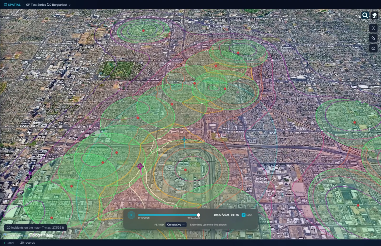
The map your data deserves, with the licensing question already answered.
A world basemap ships inside the application, so the globe draws with no network connection at all. Everything above that is your choice, and the free choice is a good one.
- 01United States imagery, free. Records default to USGS aerial imagery: public domain, no key, no royalty, no shared quota. A USGS street map is there too, roads and names on a light ground, for when a map has to look like a map.
- 02Photorealistic 3D on your Google key. Buildings, trees and terrain as they stand, and your points settle onto the ground as the city sharpens.
- 03Your agency's ArcGIS license works as it is. Save the key and the globe switches to Esri imagery straight away. A Cesium ion token works the same way.
- 04Flat when it has to be. One button for a 2D map, and a setting to open flat every time. Type an address and the globe shows the few blocks around it.
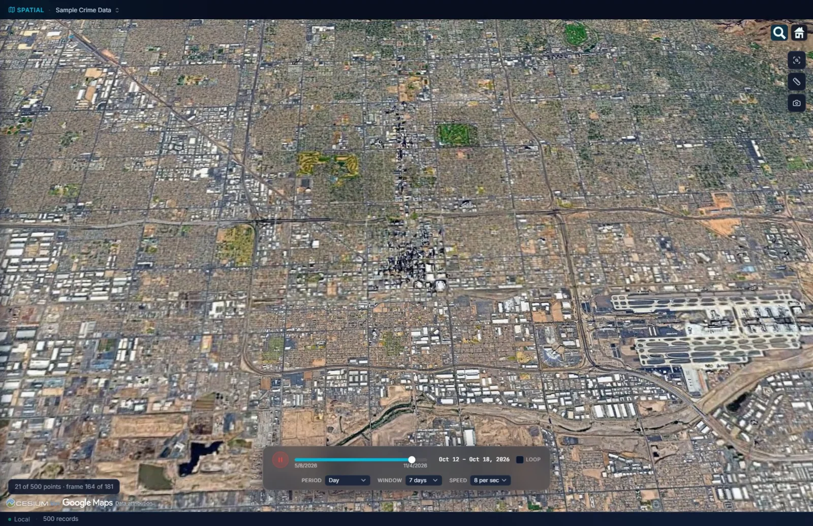
Every incident lifts to the hour it happened.
A series on a flat map is a cluster. On the globe, with time as height, it is a shape you can read: the order, the gaps, the night it went quiet.
- 01Extruded by time. Each incident rises to an altitude matching when it happened, on a thin stalk back to the ground, so earliest sits low and latest sits high.
- 02Press play. Everything up to a moment, or only the days before it, at the speed you choose. Every layer rebuilds as time advances, density included.
- 03Records with no date stay on the ground, and the map says how many. They are never dropped from the map or from a density layer because a field was blank.
- 04A 1965 cold case is a date. Dates before 1970 are dates on the globe like any other.
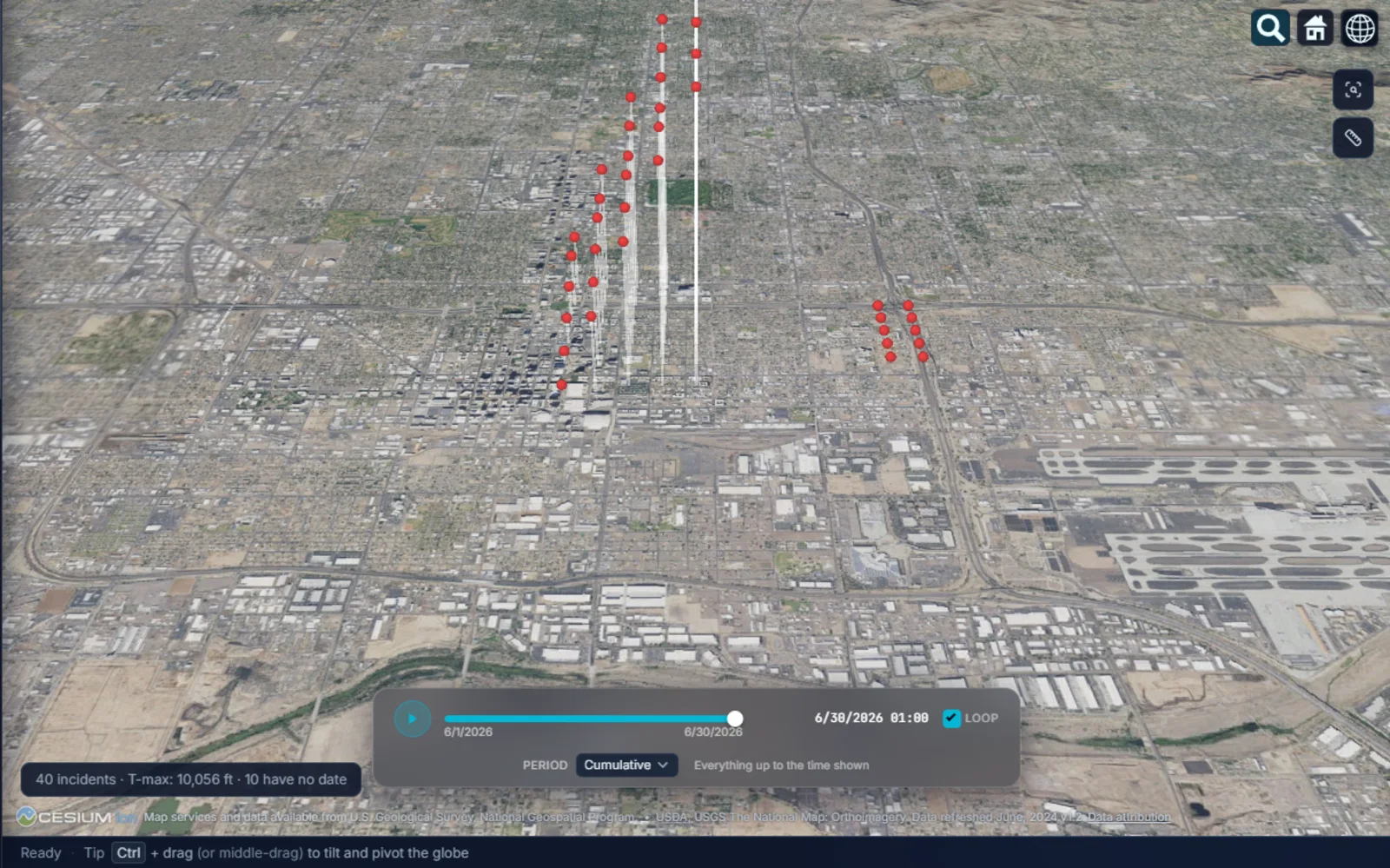
Ten analytical layers, each on or off on its own.
Points, trajectory, spider diagram, convex hull, kernel density, density clusters, heat signatures, hexbin, hot spot analysis and geographic profile. Stack any of them, and every one follows the filter on the grid.
- 01Density, hexbin, and the test on top of them. Kernel density takes its search radius from the data itself. Hexbin sums the map into prisms as tall as their counts, which keeps working where drawing every point would not. Hot spot analysis then tests those cells and draws only the ones that pass. That page has the whole argument.
- 02The spider diagram's centre tells you about the pattern. Click the yellow sphere and it gives the mean and median distance to the incidents, the standard distance, and the farthest and nearest by case number. A median well under the mean means a few far incidents are pulling the average out.
- 03The geographic profile, with its bands, rings and buffer zones, the predicted anchor as a target and the mean centre as a plus, each in a shape, colour and size of your choosing.
- 04Trajectory and convex hull for the order of a series and the ground it covers; heat signatures and density clusters that stand on the 3D ground under the incidents instead of showing through it.
Your boundaries as prisms, your places as layers, and two places in one record.
The globe is not finished until it carries what your agency already has: the beats, the districts, the camera list, the pawn shops.
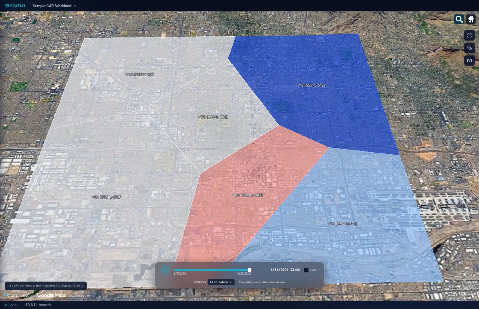
- 01Beats and districts, shaded and raised. Load them as GeoJSON, KML, KMZ or an Esri shapefile and each polygon shades by its count, or by its change against an earlier period, and extrudes to its own height.
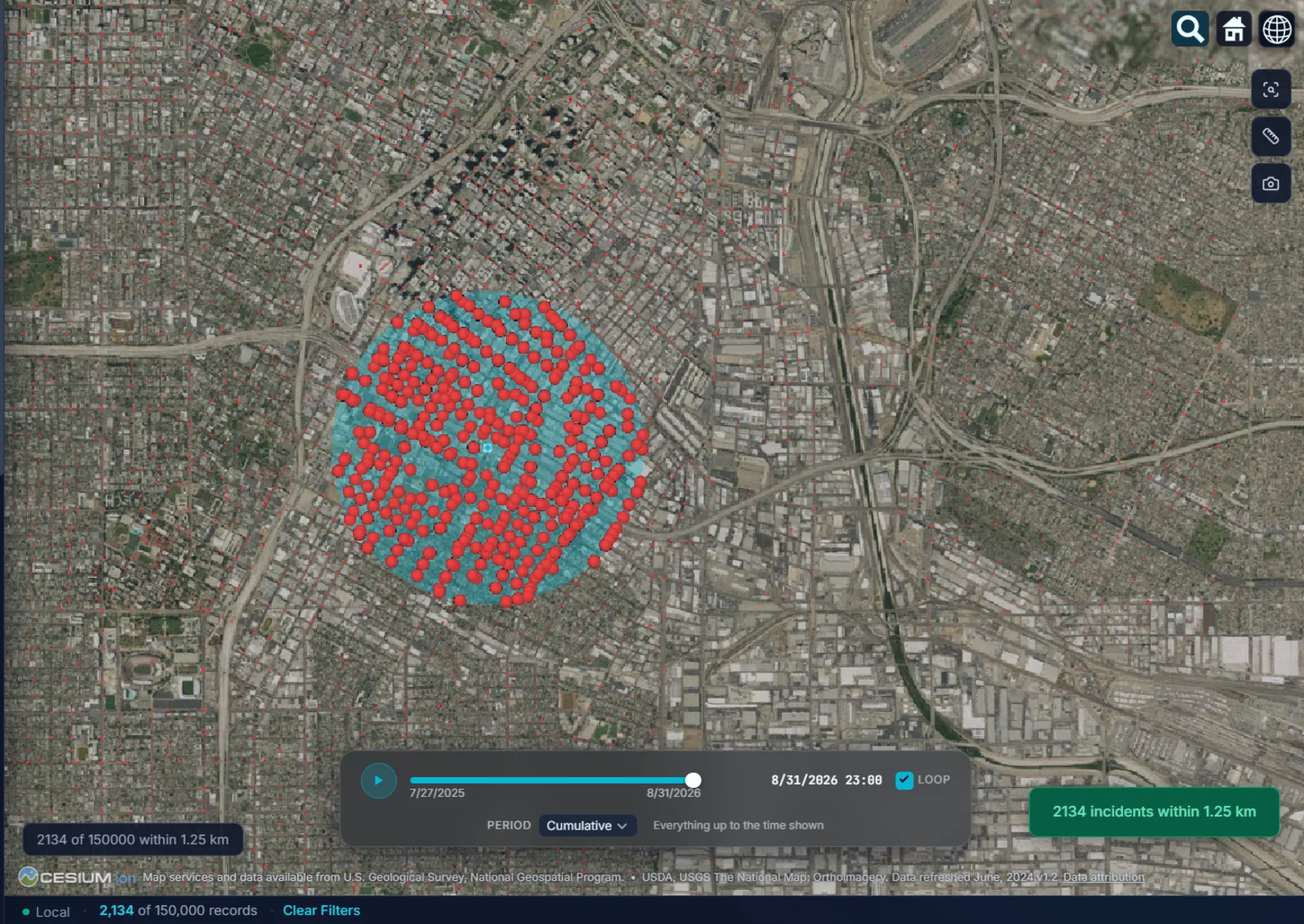
- 02Proximity search. Click a spot, drag a radius, and everything inside the circle becomes the working set for every other view: the grid, the charts, the statistics.
- 03Places as layers. Twenty-three categories of OpenStreetMap places load around your incidents, gas stations to pawn shops to schools, or load your own CSV of cameras. Every incident card ends in Near this, and the gas station canvass starts from there.
- 04Stolen to recovered. A vehicle record carries both places in one row. MICHAEL draws the arc from where it was taken to where it turned up, by distance, direction and days, and every density layer can move to the recovered end. Name the two places and the layer takes your names: Home to offense, Call to arrival.
- 05A phone's route through its cell sites, drawn as a line through the towers it used in order, which says on its face that a tower is where the phone connected and not where the phone was.
It shows you where to look.
Every layer on the globe is a way of seeing the records. None of them is a finding on its own, and the software says so where it matters.
- 01The spider centre is an average location, not a predicted home or next location. Its own card says so.
- 02The geographic profile is a probability surface, a place to look first, not an address and not a person.
- 03Density shows. The hot spot test confirms. Kernel density shows where the records are thick. Whether a thick patch means anything is the hot spot test's job, and a random scatter usually passes none of it.
- 04It asks which coordinate system you use. A file in State Plane or UTM is asked which system it is in, offered the likeliest with the reason, and converted only after you choose. Your original X and Y columns are kept.
Try it on your own data.
Fourteen days, every feature, on one machine. Tell us who you are and we will email you your own download link. Nothing to activate. Your data stays on your machine and stays yours when the trial ends. No newsletter, no drip sequence.
Built for the people who do the work Sworn agencies, crime analysis units, public safety partners, and corporate investigation teams. Workstations are $2,500 a year, everything included. Academia and nonprofits: ask about license pricing.
Or email info@sworn.ai. A person answers.